Temporal and Spatial Variation of Radiative Forcing

Also, Why RF is likely 4.1 W/m² and not 3.7 W/m²

Background

In the previous post, Mimicking Myhre, I shared how I used the Column Radiation Model (CRM) to mimic ( if not replicate ) the Myhre et. al. calculations for Radiative Forcing (RF) which has been the standard reference for the IPCC. The concept of RF, as defined by the IPCC, is

“Radiative forcing is the change in the net, downward minus upward, radiative flux ( expressed in W/m^2 ) at the tropopause or top of the atmosphere due to a change in an external driver of climate change, such as, for example, a change in the concentration of carbon dioxide… The traditional radiative forcing is computed with all tropospheric properties held fixed at their unperturbed values, and after allowing for stratospheric temperatures, if perturbed, to readjust to radiative-dynamical equilibrium. …”

Discussions of atmospheric profiles to use in related papers discussed whether a single global average sounding was sufficient or whether the three regional average soundings of the TREX experiment were necessary. The conclusion was that the three soundings were necessary but the global set of soundings ( from 2.5 to 10 degrees resolution ) were not. Since the time these papers were authored, archived atmospheric data of 1 degree  resolution ( which is 6.25 to 100 times as fine as those mentioned from the early 1990s ) is now publicly available. Because I was curious about how RF varied spatially and temporally, I decided to apply the CRM to the global CFS one degree analysis fields for given times.

CFS Analysis Data

The Climate Forecast System (CFS) analysis fields ( the zero hour forecast ) provide  objective analysis for most of the input fields necessary for executing the CRM. Importantly, that includes cloud amount and cloud liquid water content. By contrast, the clouds in the TREX soundings were somewhat arbitrarily prescribed. By examining the difference between the net radiance for this atmosphere at preindustrial CO2 ( 279 ppm ) and twice that, we can assess the RF across the globe and over time. For all these results, the stratosphere is cooled by recursively applying the imposed cooling rate until the cooling rate is near zero ( this is the so called ‘adjusted’ forcing ).

Seasonal Variation of RF

Figure 1 depicts the variation around the globe of adjusted RF at the tropopause on the 21st day of each month in 2010. Notice the minima at the poles and the maximum in the tropics. Also notice the effects of clouds, water vapor, temperature, and vertical profile of temperature which manifest as various feature shapes of RF variation.

Seasonal Variation of Global Average RF

Figure 2 depicts the spatially weighted global average of adjusted RF at the tropopause for the 21st day of each month in 2010. Notice the slight maximum during the Northern summer and the slight minimum duing the Northern winter, in accordance with the Northern continents impact on global average temperature. Also notice that the annual mean RF value of 4.1W/m2 is somewhat higher than the nominal value of 3.7 W/m2.

Diurnal Variation of RF

Figure 3 depicts the diurnal variation of RF for 0Z, 6Z, 12Z, and 18Z on March 21, 2010. Notice the subtle decrease of RF which tracks from East to West in the animation. This signifies the reduction of shortwave radiance at the tropopause for the portion of earth for which the sun is most direct.

Diurnal Variation of Global Average RF

Figure 4 depicts the spatially weighted global average of adjusted RF at the tropopause for 0Z,6Z,12Z, and 18Z on March 21st, 2010. There is a discernable but very slight variation between RF at 0Z and RF at 12Z, possibly associated with continental influence on temperature.

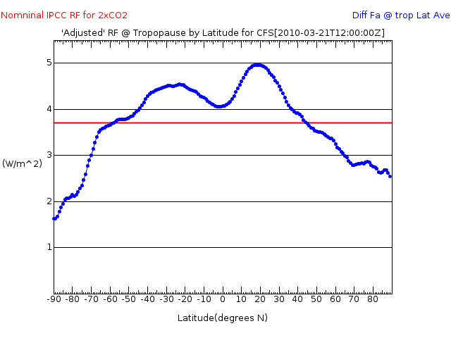
Meridional Variation of RF

Figure 5 depicts the latitude band average of adjusted RF at the tropopause on March 21, 2010. Notice the polar minima, the tropical maximum. Also notice the local tropical minima associated with the cloudiness of the Inter-Tropical Convergence Zone.

Vertical Variation of RF

Figure 6 compares the latitudinal band average of adjusted RF at the ‘Top of the Atmosphere’ ( TOA – 1 millibar level for this data ), the Tropopause, and the surface. Notice the TOA and tropopause values are very similar. Also notice the very large difference between RF at the surface and RF at the tropopause. The values of RF at the surface are even negative in the tropics. There is little variation of RF between surface and top of the atmosphere in the polar regions.

Comments

• Figure 2 does display a remarkably consistency of global average RF.
• The analysis for the CFS data does indicate a value of RF around 10% higher (4.1 W/m^2) than the nominal value (3.7 W/m^2).
• The difference is not large ( around 10% ), but it appears that the average of RF around the globe is NOT the same as the RF of the average profile, or even three average profiles.
• Both the spatial and temporal variations appear to reflect the temperature of the atmosphere. Warmer profiles, with larger radiance, incur larger reductions in radiance by CO2 doubling. Cooler profiles, with smaller radiance, incur smaller reductions in radiance by CO2 doubling.

The exact evaluation of RF is probably not that significant because RF represents a ‘What If’ hypothetical. That is ‘What if the CO2 doubled while the atmosphere was held fixed?’. The atmosphere does not stand still, of course, so RF will forever remain likely but hypothetical.  In the next post, I’ll show some results of further ‘What If’ variations of RF and and important vertical aspect.