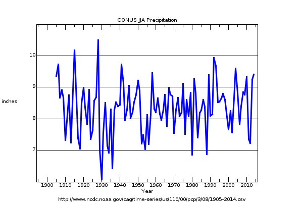
CONUS GHCN Precipitation
I looked at the GHCN Precipitation data. PRCP stations are not as prevalent, nor as old as the temperature stations so shorter time frame, since 1930, includes these stations:
Global Extreme Heat in the GHCN
After examining the record of CONUS stations in the GHCN TMAX record, it is quite reasonable to ask ‘What about the global record?’ I looked the global GHCN data ( excluding the US stations, which dominate the record, especially early on ).
When examining these data,
- Duration of record ( to compare trends in the context of other changes )
- Continuity of record ( to avoid bias from transient stations )
- Spatial coverage ( to capture regional changes )
- Representative distribution of stations
- Reliable data
Further qualities which are not necessarily known from the record are accuracy and being free of biases.

CO2 and the Last Glacial Maximum
Introduction
Often in the context of Anthropogenic Global Warming (AGW), comparisons are made to the changes of CO2 during the glacial cycles. Running the CRM models as in the last post, I compared runs for the Last Glacial Maximum and with variations holding a single component fixed in order to compare relative significance of glacial ice ( using 2010 instead of LGM ), CO2 ( using PreIndustrial instead of LGM ), Land Mask ( using 2010 land instead of the 5% increased land surface area from the LGM sea level fall ), and Orbit ( using the LGM orbit instead of LGM ).
Global Warming in the Context of Glacial Cycles
Synopsis
Using the Column Radiation Model, GFS analysis data for 2010, CERES derived surface albedo, and Last Glaical Maximum (LGM) ice and land mask estimates, it is possible to compare resulting net radiance for a number of scenarios ( with a large number of assumptions and unknowns). From these comparisons:
- CO2 Doubling indicates a large change in global mean radiative forcing(RF)
- The glacials and inter-glacials indicate relatively little change in global mean RF
- The glacials and inter-glacials appear to be a result of max RF, not global mean
- CO2 Doubling RF change is greatest at the equator, least at the poles
- The LGM RF gradients had the highest mean but lowest range
- The interglacial RF gradients exhibited the greatest range
- Both factors are consistent with dry glacials and wet interglacials
- The RF gradients for a CO2 Double do not indicate much change
- The RF gradients for a CO2 Double with no sea ice do indicate a summer reduction
‘Global Warming’ not ‘Climate Change’?
Global Warming Appears Likely
As countless papers have demonstrated, the increased opacity from increased carbon dioxide tends to impose a surplus of radiative energy which, if not reversed by strong negative feedback, would tend to accumulate, raising temperatures until radiative balance is again restored. This appears to be the case when calculated for nearly all the various vertical atmospheric profiles, with the possible exception of the high Antarctic where increased carbon dioxide leads to net radiative deficit. There are ways other than warming in which the atmosphere might reverse some of the radiative imbalance imposed by GHGs, but the fact that the vast majority of observed atmospheric profiles appear radiatively sensitive to GHG increase appears to make continued warming likely with continued increases in carbon dioxide. Continue reading
Upper Air Update Through 2015
With 2015 in the books, I updated a couple of plots I monitor of MSU data and RAOB ( RATPAC ) data. There’s been some discussion about the Hot Spot missing because of the cooling trend in the Eastern Pacific, which is evident in the GISSTEMP data: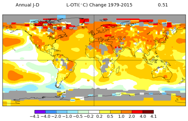
Continue reading
RATPAC and UAH, Together Again
A frustrating aspect of observing climate change is the lack of uniformity within the major global data sets. Variations of instrumentation, infrastructure, methods of observation, automation, time of observation, standards, effects of human habitation and numerous other discrepancies pollute data sets within and among comparisons.
I was recently confronted with these issues doing a simple comparison of the RATPAC radiosonde data and the UAH LT temperature trends. Below is a sample of the RATPAC trends at 700 mb versus the UAH-LT (v6) for 1979 through 2014. The RATPAC values are calculated by an ordinary least squares linear regression of the monthly anomalies. Continue reading
The Distribution of Water Vapor Changes Radiative Forcing
Continuing with runs of CRM, I recently set up a comparison of water vapor. In this comparison are runs of increased water vapor for the entire troposphere and then for just the lowest two levels. For these runs, dewpoint depression is chosen to keep the total precipitable water similar between the two distributions.
Continue reading

You must be logged in to post a comment.